Bonus lessons are optional.
A regression line
Let's continue with the goatathalon data from the last lesson.
Say you have a new goat, Billy. His running time is 90. Can we predict what his swimming time will be?
Prediction is a big thing in business analytics. Predicting sales for a new product, sales in a new region, labor costs over time... many applications.
That's where regression comes in. It's a statistical technique that gives you a formula for estimating one variable from others. We'll use linear regression, the simplest and most common form.
The technique will give us a formula like:
swimming = m * running + c
This is the formula for a straight line. m and c are constants, like:
swimming = 2 * running + 1
If these values were real, it would mean a goat could swim about half as fast as it runs, and a bit. So if a goat runs a distance in 30 seconds, we would predict it would take 2 * 30 + 1 = 61 seconds to swim the distance.
So it's the constants m and c in the forumla...
swimming = m * running + c
... are what let you make predictions. The regression method estimates m and c, from a data set. When you have them, you can make predictions.
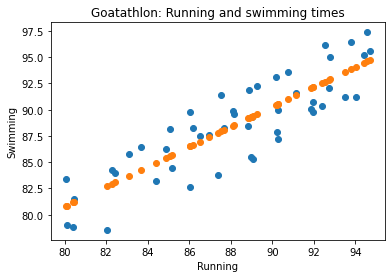
Here's what we'll make:

There are two plots. The blue one it the actual data. The orange is the predicted.
We'll take each value of running from the data set, compute the predicted value for swimming, and show it. So, we'll:
- Find values for m and c, so we have the prediction equation: swimming = m * running + c
- Loop over the records. Make a new list with the predicted swimming values for each running value.
- Call the ploty plot function twice, one for each plot we want.
Regression is a method for estimating m and c in y = m*x + c. It finds the best m and c it can, creating a line minimizing the distance of the orange points from the blue points.
Pyplot doesn't know how to compute m and c, but the Numpy package does. It's included with Sypder; nothing to download. You import it in your code, like:
- import numpy
This code will do the work. It comes after the lists for running and swimming have been made.
- m, c = numpy.polyfit(running, swimming, 1)
- predicted_swimming = []
- for run_time in running:
- prediction = run_time * m + c
- predicted_swimming.append(prediction)
- plt.scatter(running, swimming)
- plt.scatter(running, predicted_swimming)
- plt.title('Goatathlon: Running and swimming times')
- plt.xlabel('Running')
- plt.ylabel('Swimming')
- plt.show()
Line 1 computes m and c. They make the equation: predicted swimming = m * running + c. (The 1 as the last param makes it a line, rather than a quadratic, or something else.)
Line 2 makes a new list for the predicted values. Line 3 loops over all the running list. Line 4 makes the prediction for one value of running. Line 5 adds the value to the prediction list.
Line 8 plots the predicted points. The x-axis value is running, the y is predicted swimming, based on the running value.
We get:

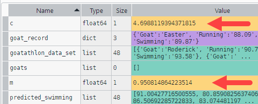
We can use the VE to find out the values of m and c:

So the formula for predicting swimming from running is:
predicted swimming = 0.95 * running + 4.7
Billy's running time is 90. His predicted swimming time is 0.95 * 90 + 4.7 = 90.2.
(Not realistic, but that's what the fake data set shows.)
AI prompt
What is linear regression? Use a goat example.
You don't have to use a goat example, but goats are cool.
Summary
- The Numpy package's
polyfitmethod computes regression coefficients. - We can use them to plot predicted values.